Date: 20 OCT 2025
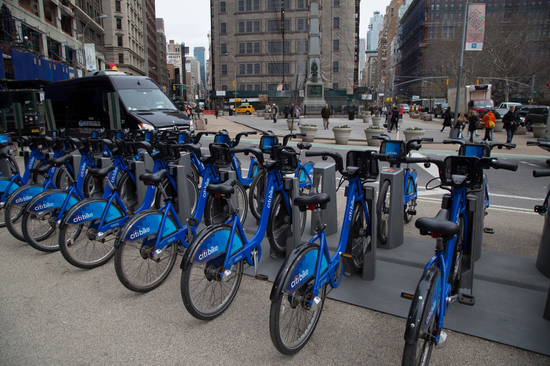
This project was completed as part of the Google Data Analytics Certificate. Cyclistic is a fictional bike-share company in Chicago. The company’s bike-share program offers 5800 bikes and 600 docking stations across the city.
The company’s financial analysis concluded that annual members bring much more profit than the casual riders. The goal for this project was to analyze Cyclistic’s 2019 bike-share data to understand how annual members and casual riders use the service differently.
For the purpose of this case study, a public dataset was provided by Motivate International Inc. The dataset is made available under their license for educational and analytical use.
I decided to use R for my analysis, as I can easily perform both the analysis and visualization in one go. The quarterly bike-share trip files for 2019 were downloaded and saved in CSV format ( data ). The dataset is split into four quarterly CSV files (Q1–Q4). Each file contains trip-level records with variables such as trip ID, bike ID, start/end time, station information, user type, gender, and birth year.
Inspecting the data: The dataset was published by an official operator and reflects actual usage. It consists of raw trip records covering the entire 12 months of 2019. No privacy concerns arise because personally identifiable information (PII) is excluded; only anonymized trip‑level data are provided. However, the dataset does not capture external factors such as weather, socioeconomic differences, or riders who choose not to disclose their gender or birth year. Consequently, the analysis was conducted with these limitations in mind, and the results do not account for these factors.
Data Integrity: Several steps were taken to ensure data’s integrity
Results After Cleaning:The total number of rides prior to cleaning was 3,818,004 and the final combined dataset consisted of 3,816,142 rows (only 1,862 rows removed, which is around 0.05%).
Missing values check: No missing values in trip ID, times, stations, or user type. Birth year missing for about 537,796 records (age also missing accordingly).
Final dataset columns: trip_id, start_time, end_time, bike_id, start_station_name, start_station_id, end_station_name, end_station_id, user_type, gender, birthyear, quarter, ride_length_seconds, ride_date, ride_year, ride_month, ride_day_of_week, ride_hour, age, age_group.
Business Question: How do annual members and casual riders use Cyclistic bikes differently? The following represent usage patterns and key insights:
Total rides:
Daily Usage Patterns:
Monthly Usage Patterns:
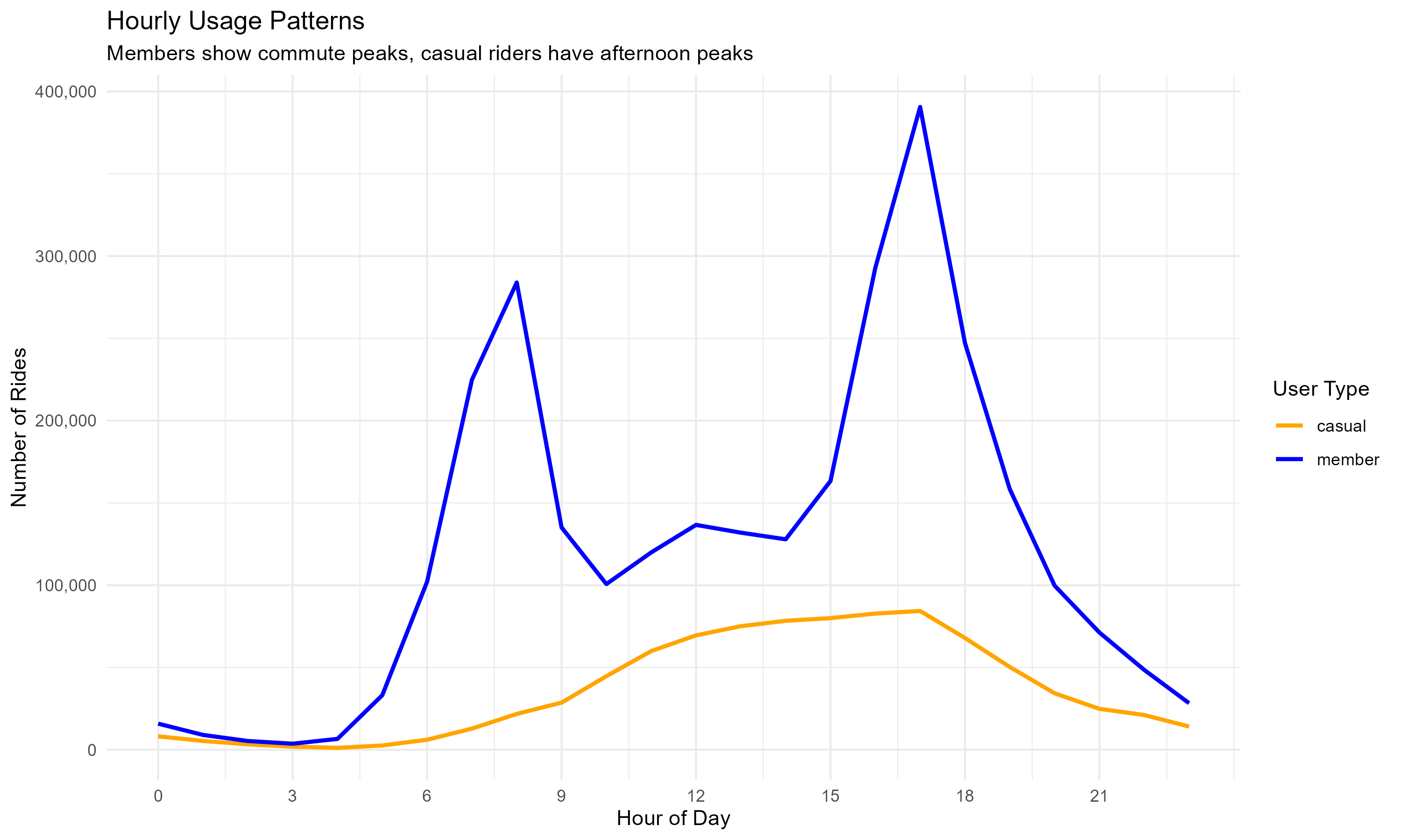
Hourly Usage Patterns:
Summary of Findings:
The insights reveal clear behavioral differences: members are commuters, casual riders are leisure users.This helps Cyclistic design targeted marketing strategies:
Key Recommendations:
# STEP 2: CLEAN AND STANDARDIZE QUARTER 1 DATA
# =============================================================================

cat("\nSTEP 2: Cleaning Quarter 1 data (January-March)...\n")

# First, let's see what columns we have in Q1
cat("Original columns in Q1:", paste(names(Q1), collapse = ", "), "\n")

quarter_1_cleaned <- Q1 %>%
  # Clean column names (makes them consistent and lowercase)
  clean_names() %>%
  # Remove completely empty rows (where all values are NA)
  dplyr::filter(!if_all(everything(), is.na)) %>%
  # Rename columns to standard names
  rename(
    trip_id = trip_id,
    bike_id = bikeid,
    start_time = start_time,
    end_time = end_time,
    trip_duration = tripduration,
    start_station_name = from_station_name,
    start_station_id = from_station_id,
    end_station_name = to_station_name,
    end_station_id = to_station_id,
    user_type = usertype,
    gender = gender,
    birthyear = birthyear
  ) %>%
  # Add a column to track which quarter this data came from
  mutate(quarter = "Q1")

cat("✓ Quarter 1 cleaned:", nrow(quarter_1_cleaned), "rows remaining\n")

# Remove the original Q1 data to free up memory
rm(Q1)
gc() # Garbage collection to free memory
# STEP 7: COMPREHENSIVE DATA CLEANING ON COMBINED DATASET
# =============================================================================

cat("\nSTEP 7: Comprehensive cleaning of combined dataset...\n")

#  Record initial row count
initial_row_count <- nrow(all_trips_combined)

#  Clean and transform the data
all_trips_2019 <- all_trips_combined %>%
  mutate(
    # Step 7.1: Standardize user type values
    user_type = case_when(
      user_type == "Subscriber" ~ "member",
      user_type == "Customer" ~ "casual",
      TRUE ~ user_type
    ),

    # Step 7.2: Convert to proper date/time formats
    start_time = as_datetime(start_time),
    end_time = as_datetime(end_time),

    # Step 7.3: Calculate ride duration in seconds
    ride_length_seconds = as.numeric(difftime(end_time, start_time, units = "secs")),

    # Step 7.4: Add useful date and time components for analysis
    ride_date = as.Date(start_time),
    ride_year = year(start_time),
    ride_month = month(start_time, label = TRUE),
    ride_day_of_week = wday(start_time, label = TRUE),
    ride_hour = hour(start_time),

    # Step 7.5: Clean gender column
    gender = case_when(
      is.na(gender) ~ "not_specified",
      gender == "" ~ "not_specified",
      tolower(gender) == "male" ~ "Male",
      tolower(gender) == "female" ~ "Female",
      TRUE ~ "Other"
    ),

    # Step 7.6: Clean birthyear and calculate age
    birthyear = as.numeric(birthyear),
    age = 2019 - birthyear,
    age_group = case_when(
      age < 20 ~ "Under 20",
      age >= 20 & age < 30 ~ "20-29",
      age >= 30 & age < 40 ~ "30-39",
      age >= 40 & age < 50 ~ "40-49",
      age >= 50 & age < 60 ~ "50-59",
      age >= 60 ~ "60 and over",
      is.na(age) ~ "Unknown",
      TRUE ~ "Unknown"
    )
  ) %>%
  # Step 7.7: Remove invalid records
  dplyr::filter(
    ride_length_seconds > 60,
    ride_length_seconds < 86400,
    !is.na(start_time),
    !is.na(end_time),
    !is.na(user_type),
    start_time < end_time,
    user_type %in% c("member", "casual")
  ) %>%
  # Step 7.8: Remove duplicate rides
  distinct(trip_id, start_time, .keep_all = TRUE)

# Step 3: Record final row count and calculate rows removed
final_row_count <- nrow(all_trips_2019)
rows_removed <- initial_row_count - final_row_count

# Step 4: Print summary
cat("✓ Comprehensive cleaning completed\n")
cat("Rows removed during cleaning:", rows_removed, "(", round(rows_removed / initial_row_count * 100, 1), "%)\n")
cat("Final clean dataset:", final_row_count, "rows\n")

#Reorder the colomns in the dataset
all_trips_2019 <- all_trips_2019 %>%
  select(
    trip_id,
    start_time,
    end_time,
    bike_id,
    start_station_name,
    start_station_id,
    end_station_name,
    end_station_id,
    user_type,
    gender,
    birthyear,
    quarter,
    ride_length_seconds,
    ride_date,
    ride_year,
    ride_month,
    ride_day_of_week,
    ride_hour,
    age,
    age_group
  )

# View the dataset
View(all_trips_2019)

# STEP 8: CHECK DATA QUALITY
# =============================================================================

cat("\nSTEP 8: Checking data quality...\n")

# Check for missing values in each column
missing_data_summary <- sapply(all_trips_2019, function(x) sum(is.na(x)))
cat("Missing values by column:\n")
print(missing_data_summary)

# Check member vs casual distribution
user_type_summary <- all_trips_2019 %>%
  count(user_type) %>%
  mutate(percentage = n / sum(n) * 100)

cat("\nUser type distribution:\n")
print(user_type_summary)

# Check date range
date_range <- range(all_trips_2019$ride_date)
cat("\nDate range of data:", as.character(date_range[1]), "to", as.character(date_range[2]), "\n")
# ANALYSIS FOCUSED ON BUSINESS TASK
# =============================================================================

cat("\nAnalyzing differences between annual members and casual riders...\n")

# 2.1 Overall comparison
overall_comparison <- all_trips_2019 %>%
  group_by(user_type) %>%
  summarise(
    total_rides = n(),
    percent_of_total = (n() / nrow(all_trips_2019)) * 100,
    avg_duration_min = mean(ride_length_seconds) / 60,
    median_duration_min = median(ride_length_seconds) / 60,
    .groups = 'drop'
  )

cat("OVERALL COMPARISON:\n")
print(overall_comparison)


# 2.2 Daily usage patterns
daily_usage <- all_trips_2019 %>%
  group_by(user_type, ride_day_of_week) %>%
  summarise(
    number_of_rides = n(),
    avg_duration_min = mean(ride_length_seconds) / 60,
    .groups = 'drop'
  )

cat("daily_usage:\n")
print(daily_usage)

# 2.3 Monthly usage patterns
monthly_usage <- all_trips_2019 %>%
  group_by(user_type, ride_month) %>%
  summarise(
    number_of_rides = n(),
    .groups = 'drop'
  )

cat("monthly_usage:\n")
print(monthly_usage)

# 2.4 Hourly usage patterns
hourly_usage <- all_trips_2019 %>%
  group_by(user_type, ride_hour) %>%
  summarise(
    number_of_rides = n(),
    .groups = 'drop'
  )

cat("hourly_usage:\n")
print(hourly_usage)
# VISUALIZATIONS FOR BUSINESS TASK
# =============================================================================

cat("\nCreating visualizations for business report...\n")

# Set clean theme
theme_set(theme_minimal())

# Visualization 1: Number of rides by day of week
plot1 <- daily_usage %>%
  ggplot(aes(x = ride_day_of_week, y = number_of_rides, fill = user_type)) +
  geom_col(position = "dodge") +
  labs(
    title = "Number of Rides by Day of Week",
    subtitle = "Comparison between annual members and casual riders",
    x = "Day of Week",
    y = "Number of Rides",
    fill = "User Type"
  ) +
  scale_y_continuous(labels = comma) +
  scale_fill_manual(values = c("casual" = "orange", "member" = "blue"))

print(plot1)

# Visualization 2: Average ride duration by day of week
plot2 <- daily_usage %>%
  ggplot(aes(x = ride_day_of_week, y = avg_duration_min, fill = user_type)) +
  geom_col(position = "dodge") +
  labs(
    title = "Average Ride Duration by Day of Week",
    subtitle = "Casual riders take longer trips on average",
    x = "Day of Week",
    y = "Average Duration (minutes)",
    fill = "User Type"
  ) +
  scale_fill_manual(values = c("casual" = "orange", "member" = "blue"))

print(plot2)

# Visualization 3: Monthly usage patterns
plot3 <- monthly_usage %>%
  ggplot(aes(x = ride_month, y = number_of_rides, color = user_type, group = user_type)) +
  geom_line(size = 1) +
  labs(
    title = "Monthly Ridership Patterns in 2019",
    subtitle = "Seasonal trends for members and casual riders",
    x = "Month",
    y = "Number of Rides",
    color = "User Type"
  ) +
  scale_y_continuous(labels = comma) +
  scale_color_manual(values = c("casual" = "orange", "member" = "blue")) +
  theme(axis.text.x = element_text(angle = 45, hjust = 1))

print(plot3)

# Visualization 4: Hourly usage patterns
plot4 <- hourly_usage %>%
  ggplot(aes(x = ride_hour, y = number_of_rides, color = user_type)) +
  geom_line(size = 1) +
  labs(
    title = "Hourly Usage Patterns",
    subtitle = "Members show commute peaks, casual riders have afternoon peaks",
    x = "Hour of Day",
    y = "Number of Rides",
    color = "User Type"
  ) +
  scale_y_continuous(labels = comma) +
  scale_x_continuous(breaks = seq(0, 23, by = 3)) +
  scale_color_manual(values = c("casual" = "orange", "member" = "blue"))

print(plot4)